From CCD Arrays, Cameras and Displays, G.C. Holst, Second Edition, 1998.
Noise:
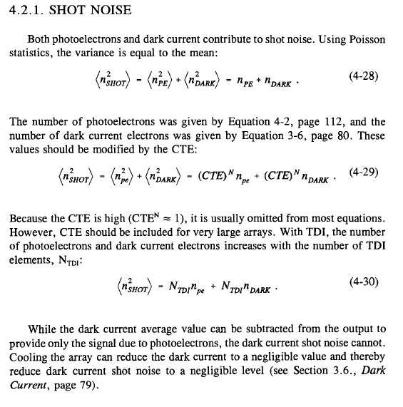
Shot noise is due to the discrete nature of electrons. It occurs when photoelectrons are created and when dark current electrons are present. Additional noise is added when reading the charge (reset noise) and introduced by the amplifier (1/f noise and white noise). If the output is digitized, the inclusion of quantization noise may be necessary. Switching transients that are coupled though the clock signals also appear as noise. It can minimized by good circuit design.

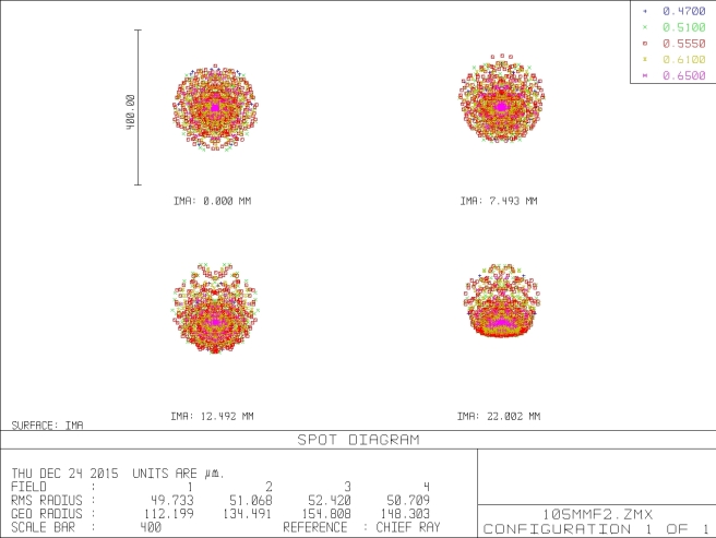
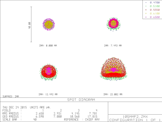
Although the origins of the noise sources are different, they all appear as variations in the image intensity. Figure 4-12a illustrates the ideal output of the on-chip amplifier before correlated double sampling. The array is viewing a uniform source and the output of each pixel is identical. Photon shot noise produces a temporal variation in the output signal that is proportional to the square root of the signal level in electrons. Each pixel output will have a slightly different value (Figure 4-12b).
Different sources of noise affecting output

Under ideal conditions, each pixel would have the same dark current and this value is subtracted from all pixels leaving the desired signal (see Section 3.6., Dark Current, page 79). However, dark current also exhibits fluctuations. Even after subtracting the average value, these fluctuations remain and create fixed pattern noise (Figure 4-12c). The output capacitor is reset after each charge is read. Errors in the reset voltage appear as output signal fluctuations (Figure 4-12d). The amplifier adds white noise (Figure 4-12e) and 1/f noise (Figure 4-12t). Amplifier noise affects both the active video and reset levels. The analog-to-digital converter introduces quantization noise (Figure 4-12g). Quantization noise is apparent after image reconstruction. Only photon shot noise and amplifier noise affect the amplitude of the signal. With the other noise sources listed, the signal amplitude, A, remains constant. However, the value of the output fluctuates with all the noise sources. Because this value is presented on the display, the processes appear as displayed noise. These noise patterns change from pixel-to-pixel and on the same pixel from frame-to-frame.
Pattern noise refers to any spatial pattern that does not change significantly from frame-to-frame. Dark current varies from pixel-to-pixel and this variation is called fixed pattern noise (FPN). FPN is due to differences in detector size, doping density, and foreign matter getting trapped during fabrication.
Photoresponse nonuniformity (PRNU) is the variation in pixel responsivity and is seen when the device is illuminated. This noise is due to differences in detector size, spectral response, and thickness in coatings. These “noises” are not noise in the usual sense. PRNU occurs when each pixel has a different average value. This variation appears as spatial noise to the observer. Frame averaging will reduce all the noise sources except FPN and PRNU. Although FPN and PRNU are different, they are sometimes collectively called scene noise, pixel noise, pixel nonuniformity, or simply pattern noise. It is customary to specify all noise sources in units of equivalent electrons at the detector output. Amplifier noise is reduced by the amplifier gain. When quoting noise levels, it is understood that the noise magnitude is the rms of the random process producing the noise. Noise powers are considered additive.
Shot Noise:
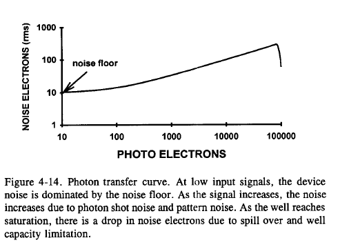
For very low photon fluxes, the noise floor dominates. As the incident flux increases, the photon shot noise dominates. Finally, for very high flux levels, the noise may be dominated by PRNU. As the signal approaches well saturation, the noise plateaus and then drops abruptly at saturation (Figure 4-14). As the charge well reaches saturation, electrons are more likely to spill into adjoining wells (blooming) and, if present, into the overflow drain. As a result, the number of noise electrons starts to decrease. Figure 4-15 illustrates the rms noise as a function of photoelectrons when the dynamic range is 60 dB. Here dynamic range is defined as NwELd < nFLOOR > . With large signals and small PRNU, the total noise is dominated by photon shot noise. When PRNU is large, the array noise is dominated by U at high signal levels.
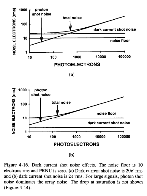
Dark current shot noise only affects those applications where the signal-to noise ratio is low (Figure 4-16). At high illumination levels, either photon shot noise or pattern noise dominates. Because many scientific applications operate in a low signal environment, cooling will improve performance. General video and industrial cameras tend to operate in high signal environments and cooling will have little effect on performance. A full SNR analysis is required before selecting a cooled camera.
Array Noise (combination of pixels):
Signal to noise plot for arrays of pixels:

Signal to noise with longer exposure time and effects of binning pixels:

Dynamic Range and pixel size relation:
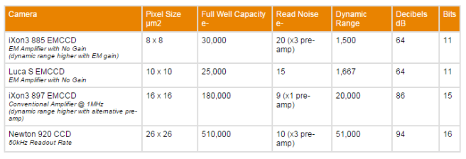
The maximum signal is that input signal that saturates the charge well and is called the saturation equivalent exposure (SEE). The well size varies with architecture, number of phases, and pixel size. The well size is approximately proportional to pixel area (Table 4-4). Small pixels have small wells.

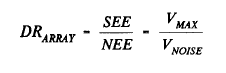
Dynamic range defined as the maximum signal (peak) divided by the rms noise. If an antibloom drain is present, the knee value is used as the maximum (See Figure 3-35, page 87). Expressed as a ratio, the dynamic range is:
Example from Andor Scientific CCD;s:
http://www.andor.com/learning-academy/dynamic-range-and-full-well-capacity-a-definition-of-ccd-dynamic-range
Other than Shot Noise:
From Nikon MicroscopyU;
https://www.microscopyu.com/articles/digitalimaging/ccdintro.html
In practice, other noise components, which are not associated with the specimen photon signal, are contributed by the CCD and camera system electronics, and add to the inherent photon statistical noise. Once accumulated in collection wells, charge arising from noise sources cannot be distinguished from photon-derived signal. Most of the system noise results from readout amplifier noise and thermal electron generation in the silicon of the detector chip. The thermal noise is attributable to kinetic vibrations of silicon atoms in the CCD substrate that liberate electrons or holes even when the device is in total darkness, and which subsequently accumulate in the potential wells. For this reason, the noise is referred to as dark noise, and represents the uncertainty in the magnitude of dark charge accumulation during a specified time interval. The rate of generation of dark charge, termed dark current, is unrelated to photon-induced signal but is highly temperature dependent. In similarity to photon noise, dark noise follows a statistical (square-root) relationship to dark current, and therefore it cannot simply be subtracted from the signal. Cooling the CCD reduces dark charge accumulation by an order of magnitude for every 20-degree Celsius temperature decrease, and high-performance cameras are usually cooled during use. Cooling even to 0 degrees is highly advantageous, and at -30 degrees, dark noise is reduced to a negligible value for nearly any microscopy application.
Providing that the CCD is cooled, the remaining major electronic noise component is read noise, primarily originating with the on-chip preamplifier during the process of converting charge carriers into a voltage signal. Although the read noise is added uniformly to every pixel of the detector, its magnitude cannot be precisely determined, but only approximated by an average value, in units of electrons (root-mean-square or rms) per pixel. Some types of readout amplifier noise are frequency dependent, and in general, read noise increases with the speed of measurement of the charge in each pixel. The increase in noise at high readout and frame rates is partially a result of the greater amplifier bandwidth required at higher pixel clock rates. Cooling the CCD reduces the readout amplifier noise to some extent, although not to an insignificant level. A number of design enhancements are incorporated in current high-performance camera systems that greatly reduce the significance of read noise, however. One strategy for achieving high readout and frame rates without increasing noise is to electrically divide the CCD into two or more segments in order to shift charge in the parallel register toward multiple output amplifiers located at opposite edges or corners of the chip. This procedure allows charge to be read out from the array at a greater overall speed without excessively increasing the read rate (and noise) of the individual amplifiers.